Learn how to use Nori to estimate how much operating life remains from a machine's sensor history.
The task: predict how much operating life remains
Predictive maintenance uses sensor readings, operating conditions, inspection records, and other historical signals to identify failure risk before an outage occurs. Teams can use that warning to inspect equipment, schedule service, or reserve capacity, whether the system is a production machine, vehicle, battery, or server fleet.
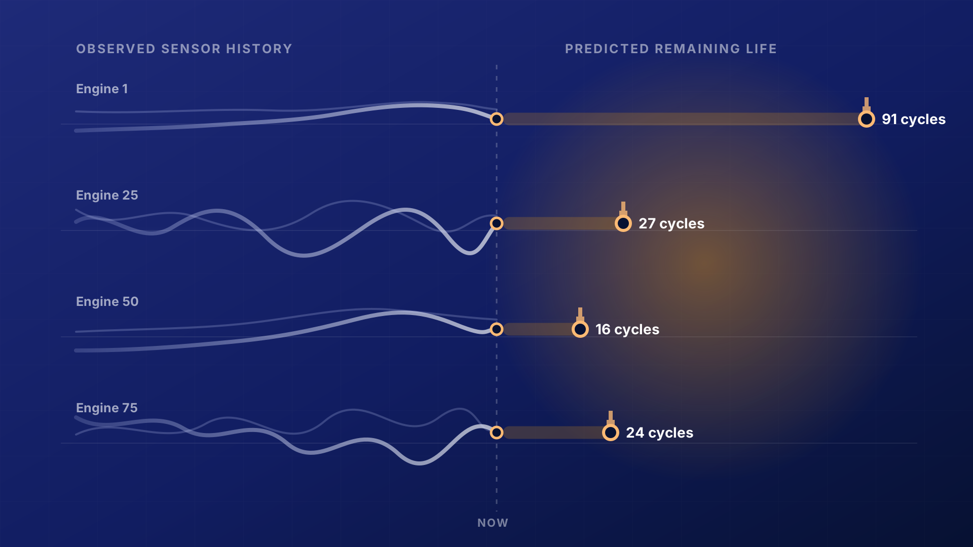
In this guide, we use one form of predictive maintenance called remaining useful life, or RUL, to answer a specific question: how many operating cycles does this system have left?
We demonstrate the approach on NASA's public FD001 turbofan simulation benchmark, which provides run-to-failure histories for 100 training engines and a separate 100-engine test fleet.
The training target is available because each training engine eventually reaches failure. At a chosen historical snapshot, RUL is the difference between the engine's final cycle and the current cycle. We cap the target at 125 cycles, a common FD001 convention that treats the early healthy region as a plateau before degradation becomes observable.
For each engine, Nori returns a continuous RUL estimate measured in operating cycles. A lower estimate means less useful operation remains, helping a team decide when to reserve a part, schedule service, rotate capacity, or retire equipment.
You can also read the sibling blog post, Better Predictive Maintenance with Nori, about failure-window prediction.
Why it has been hard
RUL prediction must infer a machine's eventual failure point from an incomplete history, often before clear signs of degradation appear. Machines can look similar early in life yet deteriorate at different rates as loads and operating conditions change, while maintenance interventions mean many assets never produce a complete run-to-failure record. A conventional workflow must turn those limited examples into a separate regression model, tune it, and retrain it as new outcomes arrive.
How Nori changes it
Nori reads machine snapshots and their known remaining lifetimes as context at inference time. It estimates a new machine's RUL from the relationships among operating conditions, sensor trajectories, and observed lifetimes, without fitting a new task-specific regressor. On this benchmark, it makes better use of those examples than the tuned XGBoost baseline.
Teams still define the RUL target, create time-aware features, and validate performance by asset. Nori removes the separate model-training and hyperparameter-search stage.
Building the context
The context table should reflect what the maintenance team knows at scoring time. We build one row for each machine snapshot, with feature columns that describe the machine's current state and how its behavior has evolved. For remaining useful life, the label records how many operating cycles remained at that snapshot.
| Machine | Operational context | Current state | Evolution through time | Nori output | ||||
|---|---|---|---|---|---|---|---|---|
| Age (cycles) | Sensor 2 current | Recent 5-cycle level (vs. history) | Recent 5-cycle shift (vs. prior 5) | vs. own history | Normalized slope | Out-of-range run | RUL prediction (cycles) | |
| Engine 58 | 176 | 643.01 | 1.46 | 0.42 | 1.49 | 0.012 | 1% | 35.8 |
| Engine 41 | 123 | 642.54 | 1.42 | 0.62 | 0.51 | 0.014 | 3% | 19.7 |
| Engine 61 | 159 | 643.29 | 1.44 | -0.20 | 2.31 | 0.014 | 3% | 21.9 |
| Engine 94 | 133 | 642.77 | 0.14 | -0.85 | 0.11 | 0.011 | 2% | 48.8 |
Figure 1 — Each row represents one machine snapshot. For FD001, three operating settings and the 14 sensor channels that change under its single operating condition feed three feature blocks: operational context describes where the machine is operating; current state captures its latest and recent behavior; and evolution through time summarizes longer-term level, direction, persistence, and volatility. Nori returns the continuous remaining-useful-life estimate, measured in operating cycles, in the final column.
The expandable snippet below shows one way to build a representative subset of the columns in Figure 1.
View the feature-building code snippet
1import numpy as np
2
3def operational_context(snapshot):
4    return {"age_cycles": snapshot["cycle"]}
5
6
7def current_state(sensor_2_history):
8    values = np.asarray(sensor_2_history, dtype=float)
9    center = values.mean()
10    scale = values.std() or 1.0
11    recent_5 = values[-5:]
12    previous_5 = values[-10:-5]
13    return {
14        "sensor_2_current": values[-1],
15        "sensor_2_recent_5_level": (recent_5.mean() - center) / scale,
16        "sensor_2_recent_5_shift": (recent_5.mean() - previous_5.mean()) / scale,
17    }
18
19
20def evolution_through_time(sensor_2_history):
21    values = np.asarray(sensor_2_history, dtype=float)
22    center = values.mean()
23    scale = values.std() or 1.0
24    standardized = (values - center) / scale
25    longest_run = run = 0
26    for outside_range in np.abs(standardized) > 2:
27        run = run + 1 if outside_range else 0
28        longest_run = max(longest_run, run)
29    return {
30        "sensor_2_vs_history": standardized[-1],
31        "sensor_2_normalized_slope": np.polyfit(np.arange(len(values)), values, 1)[0] / scale,
32        "sensor_2_out_of_range_run": longest_run / len(values),
33    }
These columns are only an illustrative subset. The benchmark also measures the share of recent observations outside the machine's earlier normal range, along with longer-history direction, persistence, and volatility. Engineering knowledge, exploratory findings, known degradation or failure mechanisms, and research from the problem domain can suggest additional features that make degradation easier to recognize. Across the 14 changing sensors and operating context, the resulting table contains 172 numeric inputs.
The exact summaries will vary by system. Rotating equipment may use vibration bands, crest factor, or spectral kurtosis; batteries may use capacity fade, resistance growth, charge-rate exposure, and thermal excursions; server fleets may use saturation duration, load slope, error bursts, and restart frequency. The transferable idea is to turn a changing history into a fixed row that captures the patterns relevant to the system.
How to predict remaining life with Nori
Nori performs tabular regression through in-context learning. Its fit() call stores the labeled machines as context.
1from synthefy_nori import NoriRegressor
2
3model = NoriRegressor(
4    model="nori-6m",
5    # Optional for datasets with free-text alert or maintenance fields:
6    # text_columns=["recent_alerts", "technician_notes"],
7)
8model.fit(X_train, remaining_cycles.astype(float))
9rul_prediction = model.predict(X_test, output_type="mean")
FD001 is numeric-only, so the optional text setting stays disabled for this benchmark. On another dataset, repeated alarm codes can be categorical columns, while free-form alerts, log excerpts, or technician notes can be named with text_columns; Nori handles their text preprocessing internally.
For comparison, XGBoost receives the same table and is tuned on the training fleet before evaluation.
Nori beats the XGBoost baseline
Nori reaches 8.77 cycles MAE, compared with 12.80 for the tuned XGBoost—a 31.5% reduction. It also lowers RMSE from 16.01 to 11.85 cycles and NASA's asymmetric penalty from 290 to 163.
Figure 2 — Results on the official 100-engine test fleet. Lower is better; Nori reduces MAE, RMSE, and NASA's asymmetric penalty relative to the tuned XGBoost baseline.
Because Nori uses labeled engines as context, teams can revise the examples or feature table without launching another hyperparameter search or producing a new task-specific model artifact.
The XGBoost baseline is not an untuned default. We searched 500 configurations with four-fold grouped cross-validation on the training engines, selected the best configuration there, and evaluated the official test fleet only after that choice was fixed.
Apply the same playbook beyond maintenance
This walkthrough uses engine sensor data to estimate remaining useful life, but the same playbook can apply across industries and problem types. Wherever a system produces a history of signals, teams can combine its current state, recent behavior, and longer-term evolution into one row, then use Nori to predict the outcome that drives the next decision.
Churn prediction is one example. A row for each account or user could summarize recent usage, longer-term engagement trends, support interactions, plan changes, clicks, and other relevant signals, then predict whether that customer will churn within a chosen window. Similar tables could support incident prediction, fraud detection, delivery-risk scoring, and many other operational decisions.
These are only a few possibilities. We're always interested in learning about novel ways teams are using Nori. Join us on Discord and tell us what you're building.
Run the full example
- Run this post in Google Colab: Open the remaining-useful-life notebook · View the source on GitHub
- Sibling post: Better Predictive Maintenance with Nori
- Dataset: NASA Prognostics Center of Excellence repository
- Nori quickstart: docs.synthefy.com/nori/quickstart
- GitHub: github.com/Synthefy/synthefy-nori
- Model weights: huggingface.co/Synthefy
Questions? contact@synthefy.com